Ensemble Learning : Enhance Your Machine Learning Models Performance to the Next Level

Introduction

Remember the time you bought a new phone? You didn’t just grab the first one you saw, right? You researched online, compared features, grilled your friends for opinions, and maybe even went to stores to hold a few in your hand. Why? Because you wanted the best, and you knew one source of information wouldn’t give you the whole picture. In short, you gather multiple feedback from different sources before making a decision. Ensemble learning is similar to this.

It is a widely used machine learning technique that combines several base models to produce one optimal predictive model, aiming to improve efficiency and accuracy. It provides more accuracy than a single model would give. In ensemble learning, the crucial factor is ensuring diversity among the base models. This diversity can arise either from using different algorithms or employing the same algorithms on different subsets of the data.

Types of Ensemble Methods

There are mainly four types of ensemble methods

1. Voting
2. Bagging
3. Boosting
4. Stacking

Before diving into each method, let’s understand what meta and base learners are for a better understanding of the next concepts.

• Base learners are the first level of an ensemble learning architecture, and each one of them is trained to make individual predictions.
• Meta learners, on the other hand, are in the second level, and they are trained on the output of the base learners.

Voting

The Voting technique involves combining predictions from multiple models and making a final decision based on the majority vote. In voting base models are always different.

There are three main types of voting:

1. Hard Voting: Final prediction based on majority votes.

2. Soft Voting: Each model provides a probability estimate for each class, and the final prediction is based on the average probabilities

3. Weighted Voting: In weighted voting, there is an assumption that some models have more skill than others and those models are assigned with more contribution when making predictions.

Let’s understand it by an Example

Suppose we have three classifiers: Model 1, Model 2, and Model 3, each trained on a dataset to predict whether an email is spam or not.

Model 1 predicts “Spam”

Model 2 predicts “Spam”

Model 3 predicts “Not Spam”

In hard voting, the majority class is “Spam,” so the ensemble’s final prediction is “Spam.”

In soft voting, if the models provide probability estimates:

Model 1: Prob(Spam) = 0.8, Prob(Not Spam) = 0.2

Model 2: Prob(Spam) = 0.9, Prob(Not Spam) = 0.1

Model 3: Prob(Spam) = 0.3, Prob(Not Spam) = 0.7

The average probabilities are calculated, and since the class with the highest average probability is “Spam,” the final prediction is “Spam.”

In Weighted Voting, each model’s vote is given a specific weight, and the final prediction is based on the weighted sum of the votes.

Model A: Prob(Spam) = 0.8, Prob(Not Spam) = 0.2 (Weight = 0.5)

Model B: Prob(Spam) = 0.9, Prob(Not Spam) = 0.1 (Weight = 0.2)

Model C: Prob(Spam) = 0.6, Prob(Not Spam) = 0.4 (Weight = 0.3)

The weighted average probabilities for each class are calculated as follows:

Weighted Prob(Spam) = (0.5 * 0.8) + (0.2 * 0.9) + (0.3 * 0.6) = 0.57

Weighted Prob(Not Spam) = (0.5 * 0.2) + (0.2 * 0.1) + (0.3 * 0.4) = 0.21

The final prediction is “ Spam “ because it has the higher weighted probability.

Bagging

Bagging is know as Bootstrap Aggregation. It is based on parallel processing that involves training multiple instances of the same base model on different subsets of the training data, promoting diversity among the base models.

In bagging, the dataset is divided into N different samples, and N models are trained using these samples, resulting in a final prediction that is typically obtained by aggregating the predictions of individual models.

For regression problems, this often involves taking the average of the predictions, while for classification, it may involve a majority vote.

Random Forest is popular algorithm that leverages bagging with decision trees as base models.

Boosting

Boosting follows a sequential approach, where the prediction of the current model influences the next one. Each model in the boosting process iteratively concentrates on observations that were misclassified by the preceding/previous model. This iterative focus on the difficult-to-classify instances and helps improve the overall predictive performance of the ensemble.

Popular boosting algorithms include AdaBoost, Gradient Boosting, and XGBoost.

• AdaBoost: Short for Adaptive Boosting, it was one of the first successful boosting algorithms. It uses decision trees as weak learners and dynamically adjusts weights based on errors.
• Gradient Boosting: This family of algorithms builds models in a stage-wise fashion, optimizing an objective function using gradient descent. It’s highly versatile and can handle various tasks.
• XGBoost: Extreme Gradient Boosting is a highly efficient and scalable implementation of gradient boosting. It’s known for its speed, accuracy, and ability to handle large datasets.

Here’s how boosting works:

1. Train a base model on the entire dataset.

2. Identify and assign weights to misclassified instances.

3. Train the next model, emphasizing misclassified instances based on weights.

4. Update instance weights, giving higher importance to previously misclassified samples.

5. Repeat steps 3–4 until the desired number of models is reached.

6. Combine predictions by giving higher weight to models with better performance.

7. Achieve a boosted ensemble model with improved accuracy, particularly on challenging instances.

Stacking

Stacking is an ensemble learning technique that begins by generating first-level individual learners from the training dataset, utilizing various learning algorithms.

The predictions from the base learners are stacked together and are used as the input to train the meta learner to produce more robust predictions. The meta learner is then used to make final predictions.

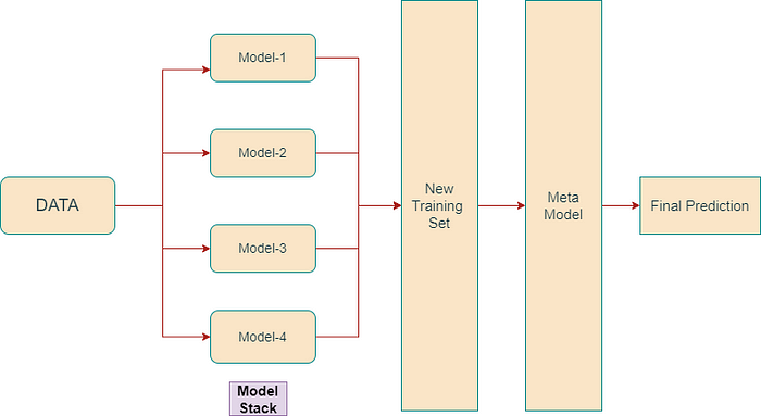
Here’s how stacking works:

1. We use initial training data to train m-number of algorithms.

2. Using the output of each algorithm, we create a new training set.

3. Using the new training set, we create a meta-model algorithm.

4. Using the results of the meta-model, we make the final prediction. The results are combined using weighted averaging.

Advantages of Ensemble Learning:

Improved Accuracy: Combining multiple models often results in higher predictive performance compared to individual models.

Robustness: Ensembles are less affected by outliers and data noise, enhancing model generalization.

Reduced Overfitting: Ensemble methods help mitigate overfitting by combining diverse models trained on different subsets of data.

Versatility: Applicable to various machine learning problems, including classification and regression.

Disadvantages of Ensemble Learning:

Complexity: Ensembles may introduce complexity, making them more challenging to interpret and analyze compared to individual models.

Computational Resources: Training multiple models can be computationally intensive, especially for large datasets.

Conclusion:

Ensemble modeling emerges as a powerful strategy that can significantly enhance the performance of machine learning models. Throughout our exploration, we delved into various ensemble learning techniques, understanding their applications in diverse machine learning algorithms. By examining their features, advantages, and disadvantages, ensemble learning proves to be a valuable approach, offering a nuanced balance between improved accuracy, robustness, and adaptability to different types of machine learning problems.